Measurements, Analyses, and Insights on the Entire Ethereum Blockchain Network

Generating Robust Counterfactual Witnesses for Graph Neural Networks

A summary of the ICDE 2024 research paper by Dazhuo Qiu, Mengying Wang, Arijit Khan, and Yinghui Wu

Background [Graph Neural Networks, Node Classification, and Explainability]: Graph neural networks (GNNs) are deep learning models designed to tackle graph-related tasks in an end-to-end manner [1]. Notable variants of GNNs include graph convolution networks (GCNs) [2], attention networks (GATs) [3], graph isomorphism networks (GINs) [4], APPNP [10], and GraphSAGE [5]). Message-passing based GNNs share a similar feature learning paradigm: for each node, update node features by aggregating neighbor counterparts. The features can then be converted into labels or probabilistic scores for specific tasks. GNNs have demonstrated their efficacy on various tasks, including node and graph classification [2], [4], [6], [7], [8], and link prediction [9].

Given a graph G and a set of test nodes V_T, a GNN-based node classifier aims to assign a correct label to each node v ∈ V_T. GNN-based classification has been applied for applications such as social networks and biochemistry [11], [12], [13].

GNNs are “black-box” — it is inherently difficult to understand which aspects of the input data drive the decisions of the network. Explainability can improve the model’s transparency related to fairness, privacy, and other safety challenges, thus enhancing the trust in decision-critical applications. Graph data are complex, noisy, and content-rich. End users and domain scientists (e.g., data scientists, business analysts, chemists) often find them difficult to query and explore. Hence, it is even more critical to provide human-understandable explanations over classification results on such datasets [14], [15] [16].

Motivation and Problem Statement [Robust Explanations]: For many GNNs-based tasks such as node classification, data analysts or domain scientists often want to understand the results of GNNs by inspecting intuitive, explanatory structures, in the form where domain knowledge can be directly applied [17]. Such explanation should indicate “invariant” representative structures for similar graphs that fall into the same group, i.e., be “robust” to small changes of the graphs and be both “factual” (that preserves the result of classification) and “counterfactual” (which flips the result if removed from G) [18]. Given a graph neural network M, a robust counterfactual witness (k-RCW) refers to the fraction of a graph G that are counterfactual and factual explanation of the results of M over G, but also remains so for any “disturbed” G by flipping up to k of its node pairs.

The need for such robust, and both factual and counterfactual explanation is evident for real-world applications such as drug design or cyber security.

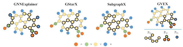
Example 1: [Interpreting “Mutagenics” with Molecular Structures]. In drug discovery, GNNs have been applied to detect mutagenicity structures, which has an adverse ability that causes mutations [31], [32]. Consider G₁ depicted in Fig. 1, which is a graph representation of a real-world molecular database [33], [34]. The nodes of G₁ refer to the atoms of the molecules, and the edges of G₁ represent the valence bonds between a pair of atoms. Given a set of “test nodes” V_T in G, a GNN-based classifier M is trained for the task to correctly assign, for each of the nodes in V_T, a label: “mutagenic”, if it belongs to a chemical compound that is a mutagenicity structure; and “nonmutagenic”, otherwise.

A natural interpretation to a chemist would be to identify a subgraph G₁ that contains most of the “mutagenic” nodes as a toxicophore structure, that is, a critical fraction of chemical compounds responsible for mutagenicity [35]. Consider the example in Figure 1. On the left is a mutagenic molecule due to the bold nitro group. Meanwhile, the remaining structure after removing the nitro group is considered as non-mutagenic. However, considering a similar molecule that only misses two bonds (dotted edges), which is in the middle, the red bold structure is an aldehyde with a high risk of triggering mutagenicity. To ensure that the discovered mutagenic-related chemical compounds are meaningful to a family of molecules, it is required to find a robust explanation structure, such as the bold indicated structure on the right molecule.

Existing GNN explanation methods may return different structures as the test nodes vary or carry “noisy” structures such as carbon rings or hydrogen atoms that are not necessarily corresponding to toxicophores (as verified in our experimental results). This may make it difficult for a chemist to discern the potential toxic structure hidden inside normal structures. (e.g., red bold aldehyde in the middle molecule of Figure 1.) Moreover, instead of analyzing explanations for each molecule, identifying a common “invariant” explanation that remains the same over a family of similar molecules with few bond differences could improve the efficiency of identifying mutagenic-related chemical compounds. A more effective approach is expected to directly compute explanation structures which are, or contain such toxicophores as robust structures, closer to what a chemist is familiar with.

Example 2: [Understanding “Vulnerable Zone” in Cyber Networks]. Graph G₂ in Fig. 1 is a fraction of a provenance graph [36]. It consists of nodes that represent files (oval) or processes (rectangle), while the edges depict access actions. The graph contains a substructure that captures a multi-stage attack. The attack is initiated by an email with a malicious attachment that is disguised as an invoice, and targets at a script “breach.sh” to perform a data breach. Attack tactics are encoded as paths or subgraphs (with red-colored, solid or dashed edges) in G₂. A valid attack path must access a privileged file (‘/.ssh/id rsa’ or ‘/etc/sudoers’) and the command prompt (‘cmd. exe’) beforehand. A GNN-based node classifier is trained to identify potential attack targets (to be labeled as “vulnerable”, colored orange in G₂) [37].

An emerging challenge is to effectively detect a two-stage tactic, which first uses, e.g., “DDoS” as a deceptive attack (via red dashed edges) on various fake targets to exhaust defense resources, to hide the intention of data breaching from an invariant set of high-value files as true target (via red solid edges). In such cases, a GNN-classifier can be “fooled” to identify a test node as “vulnerable” simply due to majority of its neighbors wrongly labeled as “vulnerable” under deceptive stage. On the other hand, a robust explanation for those correct labeling of test nodes should stay the same for a set of training attack paths. In such cases, the tactic may switch the first-stage targets from time to time to maximize the effect of deceptive attacks. As our explanation structures (RCWs) remain invariant despite various deceptive targets, they may reveal the true intention regardless of how the first stage deceptive targets change. As such, the explanation also suggests a set of true “vulnerable” files that should be protected, thereby helping mitigate the impact of deceptive attacks. In particular,

(1) There are two primary witnesses to explain the test node’s label: (‘cmd.exe’, ‘/.ssh/id rsa’, ‘breach.sh’) and (‘cmd.exe’, ‘/etc/sudoers’, ‘breach.sh’), each includes a factual path that leads to the breach and serves as evidence to explain the test node’s label as “vulnerable”.

(2) Furthermore, a CW is shown as the combined subgraph of these two witnesses, denoted as G_w2 (shaded area of G₂ in Fig. 1). Removing all edges in G_w2 from G will reverse the classification of the test node to “not vulnerable”, as the remaining part is insufficient for a breach path.

(3) G_w2 is also a k-RCW for the test node’s label, where k=3, which is the maximum length of a deceptive attack path. It indicates that for any attack path involving up to k deceptive steps, G_w2 remains unchanged. It, therefore, identifies the true important files which must be protected to mitigate the impact of deceptive attacks.

Nevertheless, computing such an explanation can be expensive due to the large size of provenance graphs. For example, a single web page loading may already result in 22,000 system calls and yields a provenance graph with thousands of nodes and edges [38], [36]. Especially for sophisticated multi-stage attacks above, it may leave complex and rapidly changing patterns in the provenance graph. Detecting and mitigating such attacks require the ability to process large amounts of data quickly for real-time or near-real-time threat analysis

Related Work [GNN Explanations]: Several approaches have been proposed to generate explanations for GNNs, [19], [20], [21], [22], [24], [23], [25], [28], [26], [27]. For example, GNNExplainer [24] learns to optimize soft masks for edges and node features to maximize the mutual information between the original and new predictions and induce important substructures from the learned masks. SubgraphX [25] employs Shapley values to measure a subgraph’s importance and considers the interactions among different graph structures. XGNN [28] explores high-level explanations by generating graph patterns to maximize a specific prediction. GCFExplainer [26] studies the global explainability of GNNs through counterfactual reasoning. Specifically, it finds a small set of counterfactual graphs that explain GNNs. CF2 [29] considers a learning-based approach to infer substructures that are both factual and counterfactual yet does not consider robustness guarantee upon graph disturbance. CF-GNNExp [23] generates counterfactual explanations for GNNs via minimal edge deletions. Closer to our work is the generation of robust counterfactual explanations for GNNs [30]. The explanation structure is required to be counterfactual and stable (robust) yet may not be a factual explanation. These methods do not explicitly support all three of our objectives together: robustness, counterfactual, and factual explanations; neither scalable explanation generation for large graphs are discussed.

Our Contributions:

(1) We formalize the notion of robust counterfactual witness (RCW) for GNN-based node classification. An RCW is a subgraph in G that preserves the result of a GNN-based classifier if tested with RCW alone, remains counterfactual (i.e., the GNN gives different output for the remaining fraction of the graph if RCW is excluded), and robust (such that it can preserve the result even if up to k edges in G are changed).

(2) We analyze properties of k-RCWs regarding the quantification of k-disturbances, where k refers to a budget of the total number of node pairs that are allowed to be disturbed. We formulate the problems for verifying (to decide if a subgraph is a k-RCW) and generating RCWs (for a given graph, GNN, and k-disturbance) as explanations for GNN-based node classification. We establish their computational hardness results, from tractable cases to co-NP hardness.

(3) We present feasible algorithms to verify and compute RCWs, matching their hardness results. Our verification algorithm adopts an “expand-verify” strategy to iteratively expand a k-RCW structure with node pairs that are most likely to change the label of a next test node, such that the explanation remains stable by including such node pairs to prevent the impact of the disturbances.

(4) For large graphs, we introduce a parallel algorithm to generate k-RCWs at scale. The algorithm distributes the expansion and verification process to partitioned graphs, and by synchronizing verified k-disturbances, dynamically refines the search area of the rest of the subgraphs for early termination.

(5) Using real-world datasets, we experimentally verify our algorithms. We show that it is feasible to generate RCWs for large graphs. Our algorithms can produce familiar structures for domain experts, as well as for large-scale classification tasks. We show that they are robust for noisy graphs. We also demonstrate application scenarios of our explanations.

For more information, click here for our paper.  Code: GitHub.

Blog post contributed by: Arijit Khan

References:

[1] Z. Wu, S. Pan, F. Chen, G. Long, C. Zhang, and P. S. Yu, “A comprehensive survey on graph neural networks,” IEEE Transactions on Neural Networks and Learning Systems, vol. 32, no. 1, pp. 4–24, 2020.

[2] T. N. Kipf and M. Welling, “Semi-supervised classification with graph convolutional networks,” in ICLR, 2017.

[3] P. Velickovic, G. Cucurull, A. Casanova, A. Romero, P. Lio, and Y. Bengio, “Graph attention networks,” arXiv preprint arXiv:1710.10903, 2017.

[4] K. Xu, W. Hu, J. Leskovec, and S. Jegelka, “How powerful are graph neural networks?” in ICLR, 2019.

[5] W. Hamilton, Z. Ying, and J. Leskovec, “Inductive representation learning on large graphs,” in Advances in Neural Information Processing Systems (NeurIPS), 2017, pp. 1024–1034.

[6] M. Zhang, Z. Cui, M. Neumann, and Y. Chen, “An end-to-end deep learning architecture for graph classification,” in AAAI Conference on Artificial Intelligence, vol. 32, no. 1, 2018.

[7] Z. Ying, J. You, C. Morris, X. Ren, W. Hamilton, and J. Leskovec, “Hierarchical graph representation learning with differentiable pooling,” Advances in Neural Information Processing Systems (NeurIPS), vol. 31, 2018.

[8] J. Du, S. Wang, H. Miao, and J. Zhang, “Multi-channel pooling graph neural networks.” in IJCAI, 2021, pp. 1442–1448.

[9] M. Zhang and Y. Chen, “Link prediction based on graph neural networks,” Advances in Neural Information Processing Systems (NeurIPS), vol. 31, 2018.

[10] J. Klicpera, A. Bojchevski, and S. Gunnemann, “Predict then propagate: Graph neural networks meet personalized pagerank,” in ICLR, 2019.

[11] J. You, B. Liu, Z. Ying, V. Pande, and J. Leskovec, “Graph convolutional policy network for goal-directed molecular graph generation,” Advances in Neural Information Processing Systems (NeurIPS), vol. 31, 2018.

[12] E. Cho, S. A. Myers, and J. Leskovec, “Friendship and mobility: user movement in location-based social networks,” in ACM International Conference on Knowledge Discovery and Data Mining (KDD), 2011, pp. 1082–1090.

[13] L. Wei, H. Zhao, Z. He, and Q. Yao, “Neural architecture search for gnnbased graph classification,” ACM Transactions on Information Systems, 2023.

[14] M. Du, N. Liu, and X. Hu, “Techniques for Interpretable Machine Learning”, Commun. ACM, vol. 63, no. 1, 2020.

[15] Z. C. Lipton, “The Mythos of Model Interpretability”, Commun. ACM, vol. 61, no. 10, 2018.

[16] H. Yuan, H. Yu, S. Gui, and S. Ji, “Explainability in graph neural networks: A taxonomic survey,” IEEE Transactions on Pattern Analysis and Machine Intelligence, vol. 45, no. 5, pp. 5782–5799, 2023.

[17] T. Chen, D. Qiu, Y. Wu, A. Khan, X. Ke, and Y. Gao, “View-based explanations for graph neural networks,” in ACM International Conference on Management of Data (SIGMOD), 2024.

[18] J. Zhou, A. H. Gandomi, F. Chen, and A. Holzinger, “Evaluating the quality of machine learning explanations: A survey on methods and metrics,” Electronics, vol. 10, no. 5, p. 593, 2021.

[19] R. Schwarzenberg, M. Hubner, D. Harbecke, C. Alt, and L. Hennig, “Layerwise relevance visualization in convolutional text graph classifiers,” in Workshop on Graph-Based Methods for Natural Language Processing (TextGraphs@EMNLP), 2019, pp. 58–62.

[20] Q. Huang, M. Yamada, Y. Tian, D. Singh, and Y. Chang, “Graphlime: Local interpretable model explanations for graph neural networks,” IEEE Transactions on Knowledge and Data Engineering, 2022.

[21] M. S. Schlichtkrull, N. De Cao, and I. Titov, “Interpreting graph neural networks for NLP with differentiable edge masking,” in ICLR, 2021.

[22] D. Luo, W. Cheng, D. Xu, W. Yu, B. Zong, H. Chen, and X. Zhang, “Parameterized explainer for graph neural network,” Advances in Neural Information Processing Systems (NeurIPS), vol. 33, pp. 19 620–19 631, 2020.

[23] A. Lucic, M. A. Ter Hoeve, G. Tolomei, M. De Rijke, and F. Silvestri, “Cf-gnnexplainer: Counterfactual explanations for graph neural networks,” in Proceedings of the 25th International Conference on Artificial Intelligence and Statistics, vol. 151, 2022, pp. 4499–4511.

[24] Z. Ying, D. Bourgeois, J. You, M. Zitnik, and J. Leskovec, “Gnnexplainer: Generating explanations for graph neural networks,” Advances in Neural Information Processing Systems (NeurIPS), vol. 32, 2019.

[25] H. Yuan, H. Yu, J. Wang, K. Li, and S. Ji, “On explainability of graph neural networks via subgraph explorations,” in International Conference on Machine Learning (ICML), 2021, pp. 12 241–12 252.

[26] Z. Huang, M. Kosan, S. Medya, S. Ranu, and A. Singh, “Global counterfactual explainer for graph neural networks,” in WSDM, 2023.

[27] S. Zhang, Y. Liu, N. Shah, and Y. Sun, “Gstarx: Explaining graph neural networks with structure-aware cooperative games,” in Advances in Neural Information Processing Systems (NeurIPS), 2022.

[28] H. Yuan, J. Tang, X. Hu, and S. Ji, “Xgnn: Towards model-level explanations of graph neural networks,” in ACM international conference on knowledge discovery and data mining (KDD), 2020, pp. 430–438.

[29] J. Tan, S. Geng, Z. Fu, Y. Ge, S. Xu, Y. Li, and Y. Zhang, “Learning and evaluating graph neural network explanations based on counterfactual and factual reasoning,” in Proceedings of the ACM Web Conference 2022, 2022, pp. 1018–1027.

[30] M. Bajaj, L. Chu, Z. Y. Xue, J. Pei, L. Wang, P. C.-H. Lam, and Y. Zhang, “Robust counterfactual explanations on graph neural networks,” Advances in Neural Information Processing Systems (NeurIPS), vol. 34, pp. 5644–5655, 2021.

[31] J. Xiong, Z. Xiong, K. Chen, H. Jiang, and M. Zheng, “Graph neural networks for automated de novo drug design,” Drug Discovery Today, vol. 26, no. 6, pp. 1382–1393, 2021.

[32] M. Jiang, Z. Li, S. Zhang, S. Wang, X. Wang, Q. Yuan, and Z. Wei, “Drug–target affinity prediction using graph neural network and contact maps,” RSC advances, vol. 10, no. 35, pp. 20 701–20 712, 2020.

[33] L. David, A. Thakkar, R. Mercado, and O. Engkvist, “Molecular representations in ai-driven drug discovery: a review and practical guide,” Journal of Cheminformatics, vol. 12, no. 1, pp. 1–22, 2020.

[34] A. M. Albalahi, A. Ali, Z. Du, A. A. Bhatti, T. Alraqad, N. Iqbal, and A. E. Hamza, “On bond incident degree indices of chemical graphs,” Mathematics, vol. 11, no. 1, p. 27, 2022.

[35] J. Kazius, R. McGuire, and R. Bursi, “Derivation and validation of toxicophores for mutagenicity prediction,” Journal of Medicinal Chemistry, vol. 48, no. 1, pp. 312–320, 2005.

[36] H. Ding, J. Zhai, D. Deng, and S. Ma, “The case for learned provenance graph storage systems,” in 32nd USENIX Security Symposium (USENIX Security 23), 2023, pp. 3277–3294.

[37] T. Bilot, N. El Madhoun, K. Al Agha, and A. Zouaoui, “Graph neural networks for intrusion detection: A survey,” IEEE Access, 2023.

[38] W. U. Hassan, A. Bates, and D. Marino, “Tactical provenance analysis for endpoint detection and response systems,” in 2020 IEEE Symposium on Security and Privacy (SP), 2020, pp. 1172–1189.